Deep learning for the detection of γ-ray sources:
Bridging the gap between
simulations and observations
with multi-modal neural networks
LISTIC, Réunion AFuTé
| Author | Under the supervision of |
| Michaël Dell'aiera (LAPP, LISTIC) | Thomas Vuillaume (LAPP) Alexandre Benoit (LISTIC) |
dellaiera.michael@gmail.com
Introduction
Contextualisation
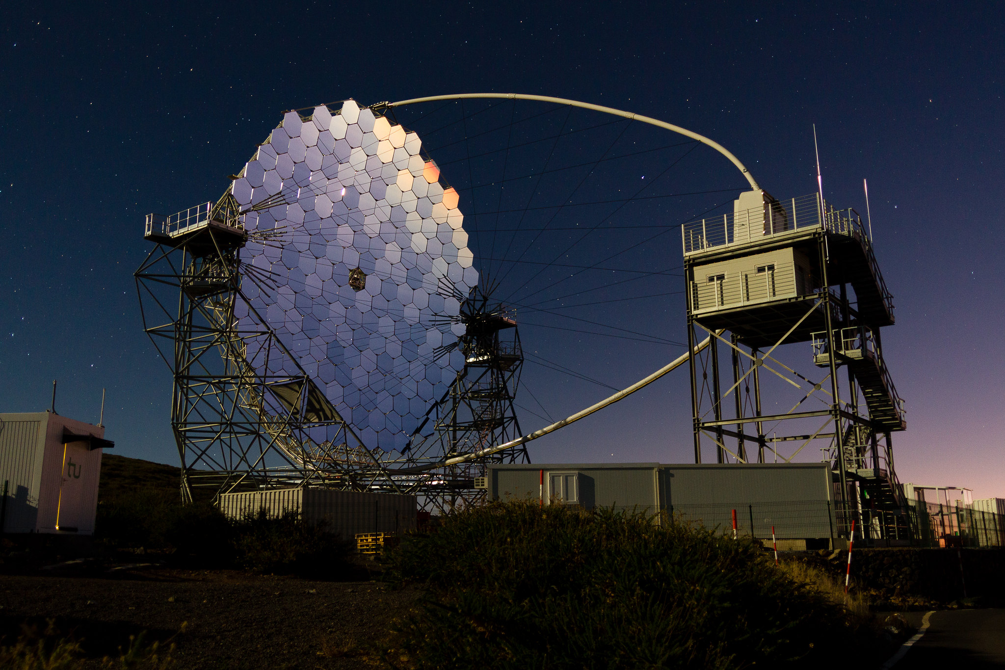
**[Cherenkov Telescope Array Observatory](https://www.cta-observatory.org/)**
* Exploring the Universe at very high energies * γ-rays, powerful messenger to study the Universe * Next generation of ground-based observatories * Large-Sized Telescope-1 (LST-1) operational
**[GammaLearn](https://purl.org/gammalearn)**
* Collaboration between LAPP (CNRS) and LISTIC * Fosters innovative methods in AI for CTA * Evaluate the added value of deep learning * [Open-science](https://gitlab.in2p3.fr/gammalearn/gammalearn)
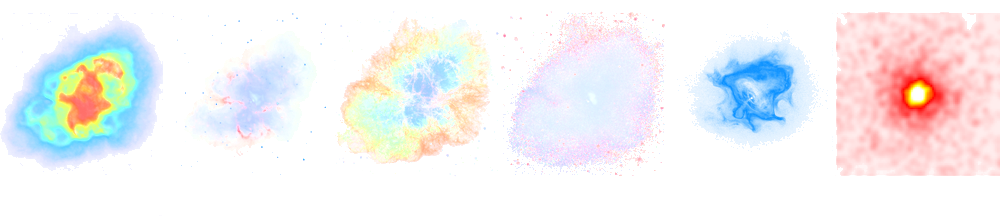
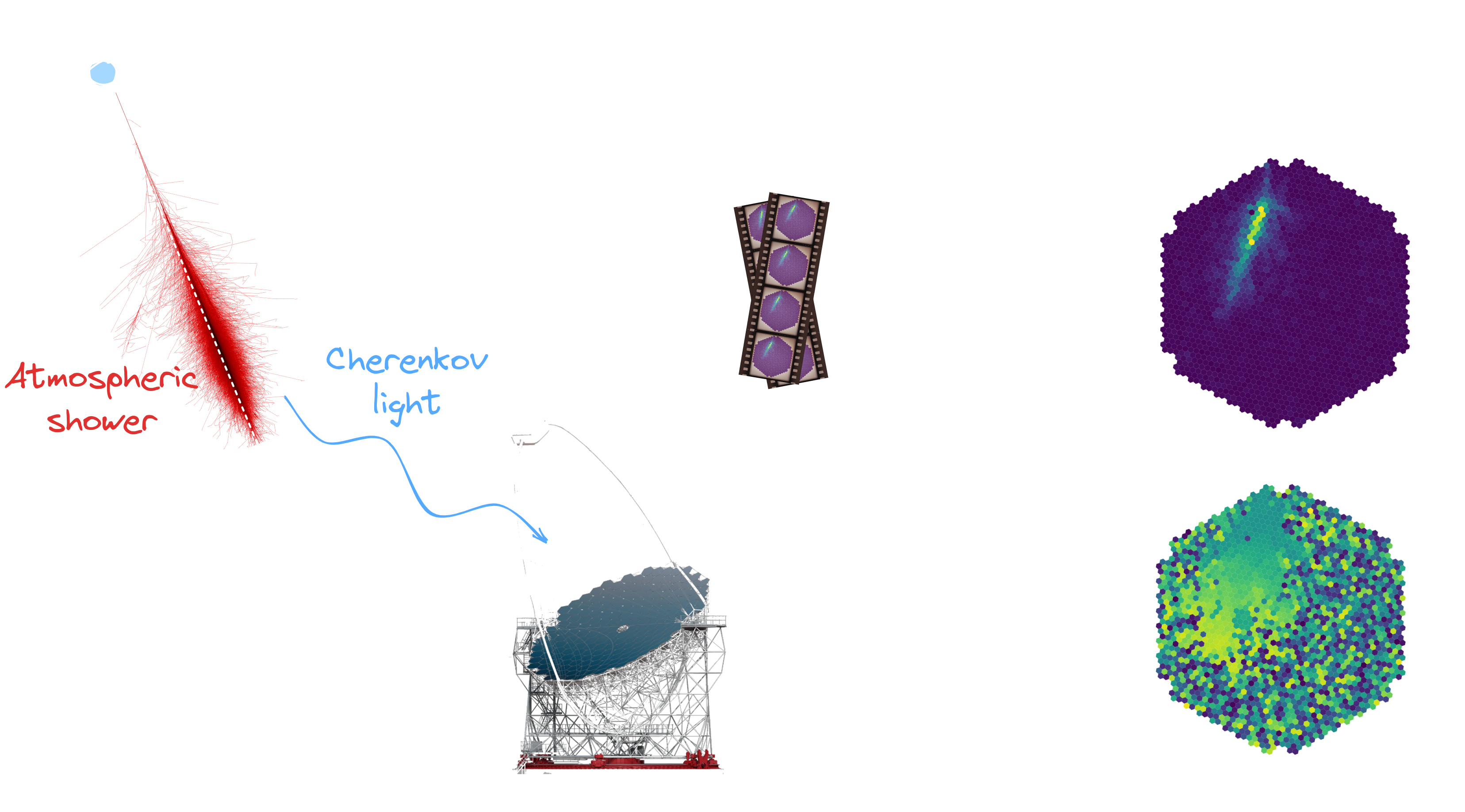
Principle of detection
Energy flux
* Many particles create atmospheric showers * Flux decreases with energy * Ratio gamma/proton < 1e-3
GammaLearn workflow
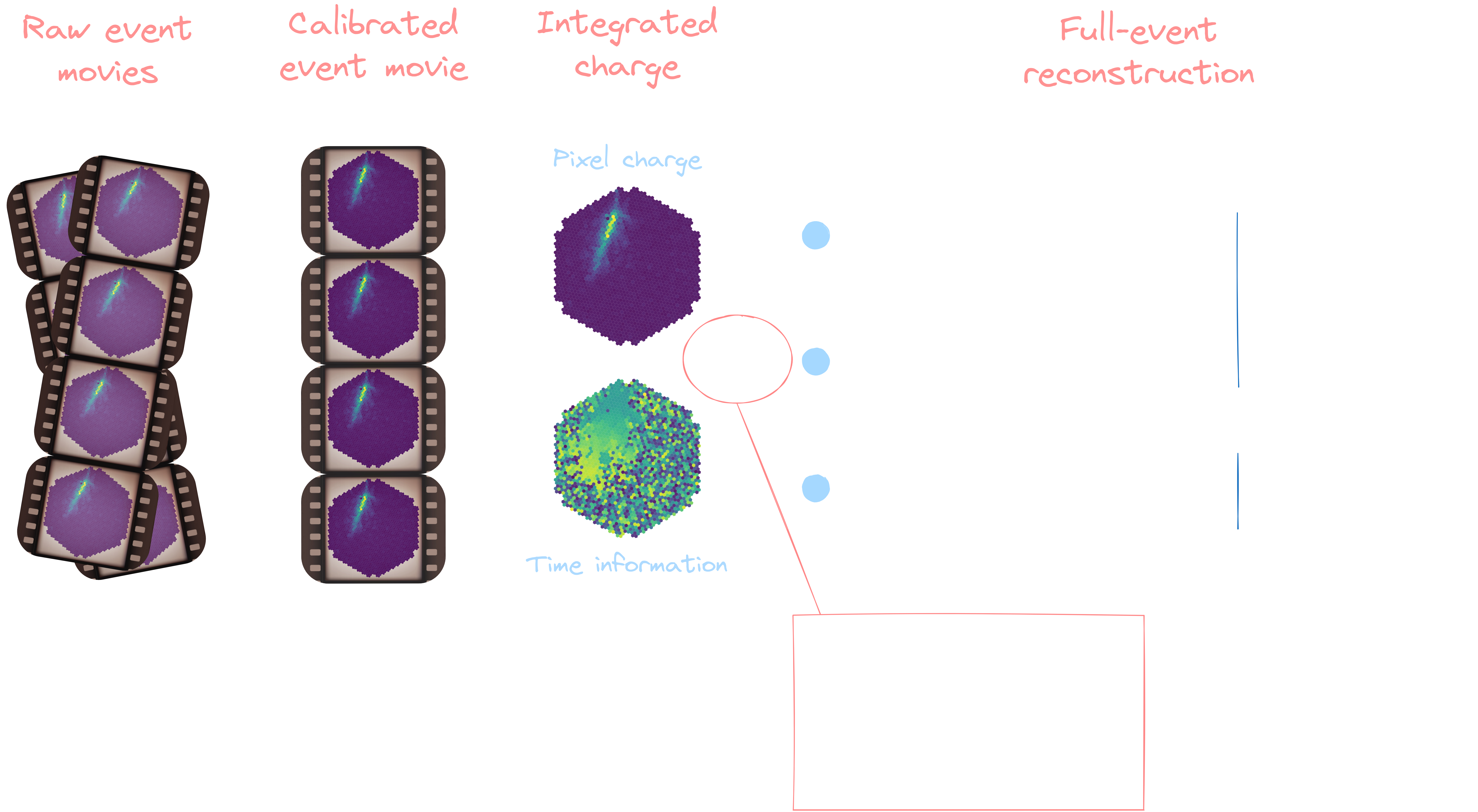
Physical attribute reconstruction
**Real labelled data are intrinsically unobtainable**
→ Training relying on simulations (Particle shower + instrument response)
* Machine learning * Morphological prior hypothesis: Ellipsoidal integrated signal * Image cleaning
GammaLearn* Deep learning (CNN-based) * No prior hypothesis * No image cleaning
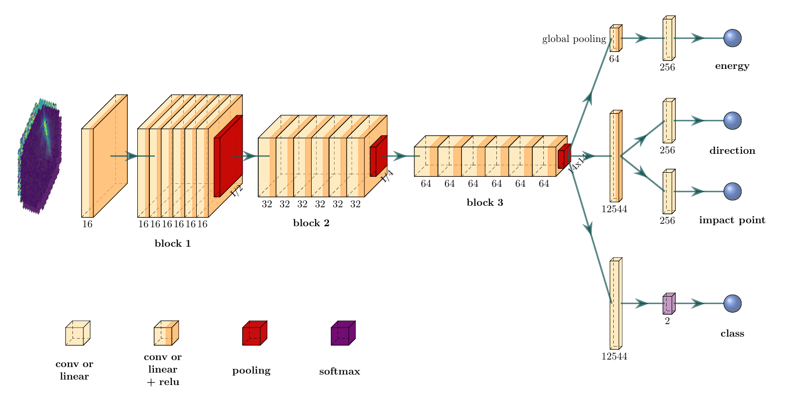
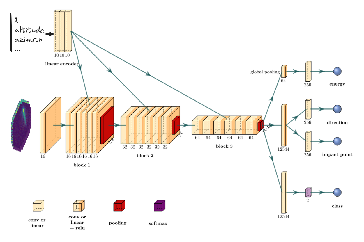
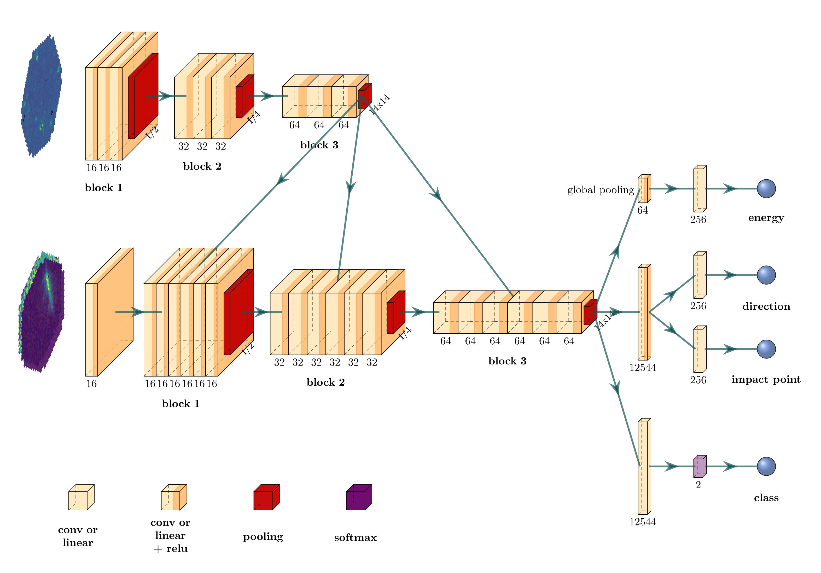
The γ-PhysNet neural network
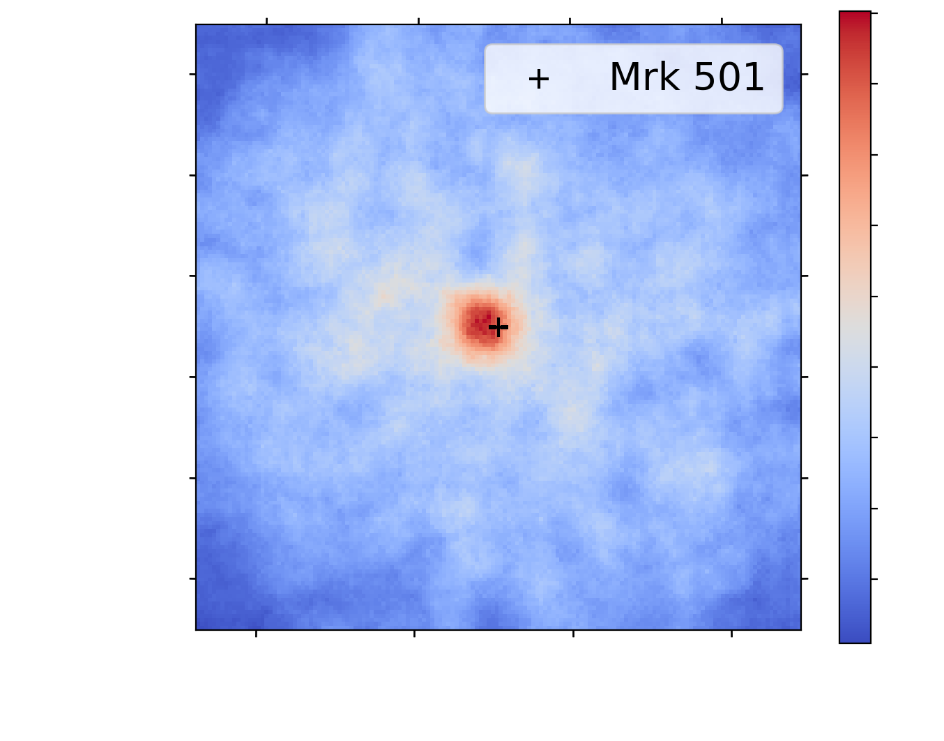
* Capability to detect a source evaluated with significance σ = f(N_γ, N_bg) * Better results with background matching → Sensitivity to background variations → Results can be improved on telescope observations
| Reconstruction algorithm | Significance (higher is better) | Background counts |
|---|---|---|
| Standard analysis + Background matching | 11.9 σ | 305 |
| γ-PhysNet | 12.5 σ | 302 |
| γ-PhysNet + Background matching | 14.3 σ | 317 |
Tab. Results on real data ([Vuillaume et al.](https://arxiv.org/abs/2108.04130.pdf))
The challenging transition from simulations to real data
Simulations and real data discrepencies
**Simulations are approximations of the reality**
Simulations and real data discrepencies
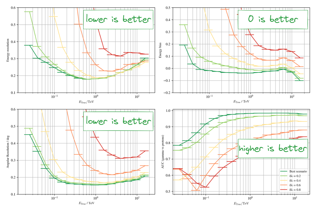
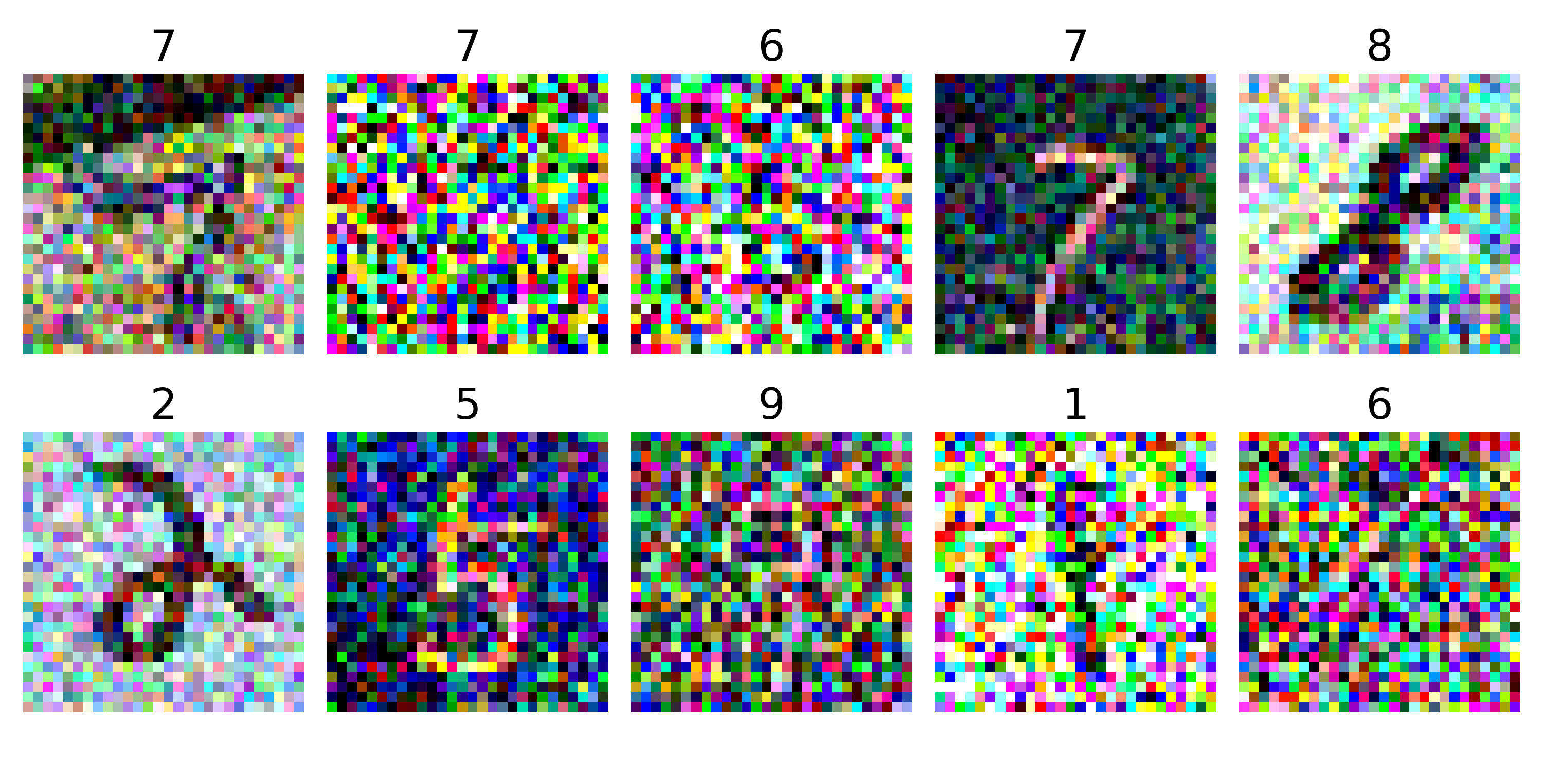
Background light from the sky: * Moonlight * Starlight * Airglow * Zodiacal light * Light pollution Main source of discreprency between simulations and real data ([Parsons et al.](https://arxiv.org/abs/2203.05315)) → Make the model robust to NSB * Data augmentation (addition of noise) noise~P(δλ) * Somehow inject the noise information within the network (δλ)
→ Approximated by Poisson distributions
Multi-modality
Multi-modality
Normalization (pre-GPU era) * Trick to stabilize and accelerate the speed of convergence * Maintains stable gradients * Diminishes initialization influence * Allows greater learning rates
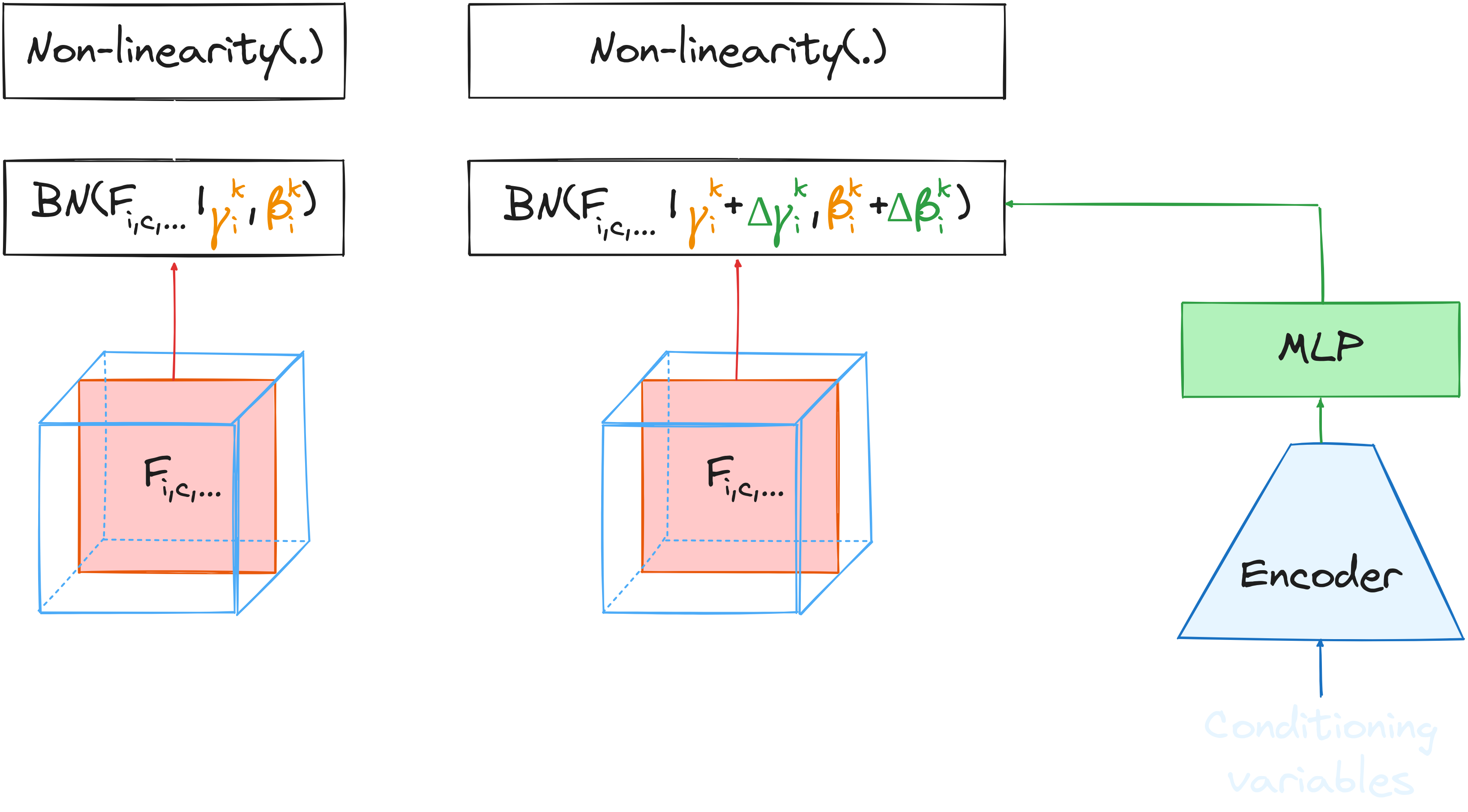
[Batch Normalization](https://arxiv.org/abs/1502.03167) (2015)
[Conditional Batch Normalization](https://proceedings.neurips.cc/paper_files/paper/2017/file/6fab6e3aa34248ec1e34a4aeedecddc8-Paper.pdf) (2017) * Elegant way to inject additional information within the network * NSB and pointing direction affects the distributions of the input data
The γ-PhysNet-CBN neural network
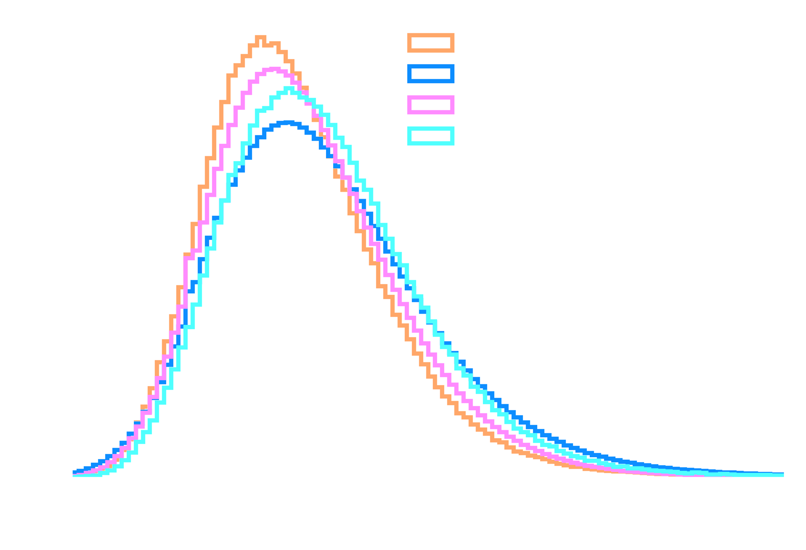
Results on simulations without CBN
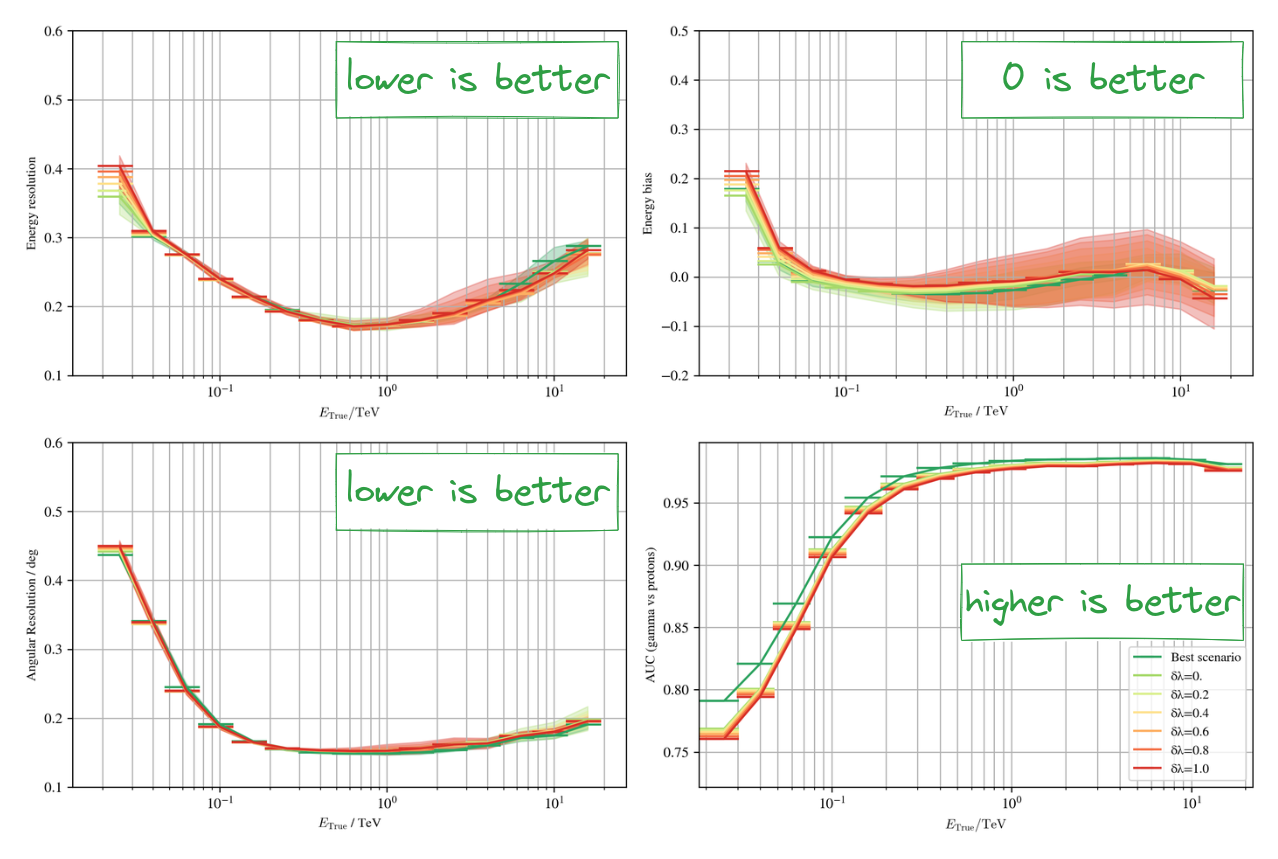
Results on simulations with CBN
Pedestal images: * Signal-free acquisitions * 100 Hz acquisition rate during observations 1. Poisson approximation * Compute Poisson rate as the pixel mean * Use it as the conditioning input 2. Direct conditioning * Use the pedestals as conditioning inputs * CNN encoder * No Poisson approximation
The γ-PhysNet-CBN neural network
* Longer trainings are required
* No miracle if information is lost
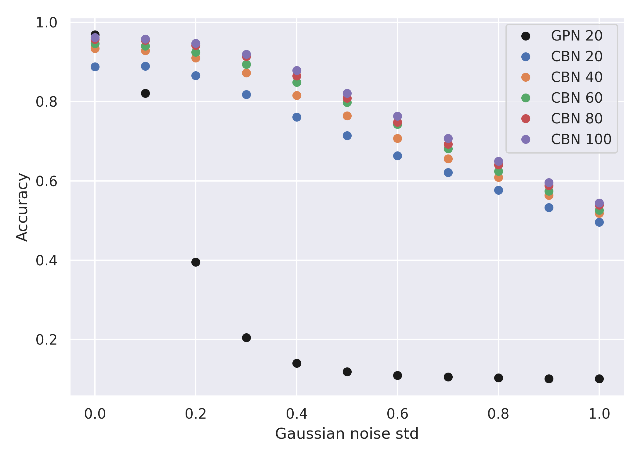
* γ-PhysNet (GPN): Trained on cleaned data, applied on noisy data * γ-PhysNet-CBN (CBN): Data augmentation
Conclusion and perspectives
Conclusion & Perspectives
- Standard analysis and γ-PhysNet strongly affected by moonlight
- Multi-modality (with CBN) is a novel technique to solve simulations vs real data NSB discreprency
- Tested on simulations
- Currently being tested on real data
- Multi-modality increases the performance in degraded conditions
- γ-PhysNet-CBN with pedestal image conditioning
- Pointing direction as auxiliar conditioning inputs
- Generalization to other sources
Acknowledgments
![]()
![]()
![]()
![]()
![]()
![]()
![]()
![]()
![]()
![]()
![]()
![]()